Application of Interval Seismic Velocities for Pre- Drill Pore Pressure Prediction and Well Design in Belayim Land Oil Field, Gulf of Suez, Egypt

A pre-drill pore pressure prediction is one of the basics for well design and the planning of well-drilling and represent a key to safe drilling and avoid drilling problems and well control operations. Knowledge of expected pore pressure will provide valuable information for efficiently drilling wells with optimum mud weights. So first we should throw light on the basic and typical terminologies used in subsurface formation pressure.

The hydrostatic pressure is the pressure exerted by the static column of fluid at a reference depth. It is dependent on the density of the formation fluid, usually water or brine, and the true vertical height of the column of fluid.

The overburden pressure is the pressure exerted at a particular depth by the weight of overlying sediments including the fluid it contains. Formation pore pressure is the pressure which formed by the fluids (formation Water, Oil, Gas) in the pore spaces of the formation. Normal formation pressure is the state where the hydrostatic column of water equal to the subsurface formation pressure.

Abnormal formation pressure is characterized by any departure from the normal trend line of any formation property depending on porosity and densities of matrix and fluid. When the formation pressure exceeding hydrostatic pressure in a specific geologic environment is defined as abnormally high formation pressure (over-pressure), Whereas formation pressure less than hydrostatic pressure is called subnormal formation pressure (Under-pressure). Figure 1 Show that schematic pressure-depth plot with the illustration of typical terminologies used in pore pressure work.

Figure 1:Schematic pressure-depth plot with illustration of typical terminologies used in pore pressure work.

A pre-drill pressure prediction using seismic velocities is based on rock physics and the analysis of seismic velocity which commonly used interval seismic velocity where the estimation of pore pressure can be obtained from transform model using seismic interval velocity to pore pressure transform. The seismic velocities should be derived using methods that give sufficient spatial resolutions, so it can be by using horizon-keyed velocity analysis for the main horizons in the section.

Determining pore pressure from interval seismic velocities is similar using the sonic log but the major difference is that the interval velocities which calculated from the RMS velocities which concerned with stacking velocities are horizontal velocities while the sonic log is measuring the vertical velocity assuming the well is vertical. In general, the vertical, the horizontal or the average. If the compaction trend is a function of vertical velocity it is important to make sure that the shale velocity is the same.

There are some of the attempts to predict pore pressure from the use of reflection seismograph data. The first pore pressure evaluation methods correlated empirically log data with pore pressure measurements, such as the equivalent depth method [1]. The pioneering work by [2] was the first method that used seismic data where found average velocity for each reflective horizon in a given survey, then the average velocities were converted to interval travel times.

Understanding the relationship between reservoir pore pressure condition and state of faulting variation for fluid flow processes in hydrocarbon migration and identify hydrocarbon migration pathways. In the present work, Eaton’s equation method was used to predict pore pressure before drilling and the results were compared with the measured Repeat Formation Tester (RFT) as a pore pressure data of the offset wells for the reliability of our results.

Geologic and structure setting of study area

The proposed area of study located in Belayim Land Oil Field which considers one of the oldest oil fields in the Gulf of Suez. Belayim Land Field is located in the eastern coast of the Gulf of Suez between longitudes 33˚ 12 and 33˚ 15 east and latitudes 28˚ 35 and 28˚ 40 north Figure 2. Belayim Land Oil Field was discovered in 1954 and occupies an area of about 113km2. From then until now continuous exploration and development efforts have been spent to raise the production to reach about 350 wells were drilled in the field, which became a very mature field and the average production rate recorded was 75000 BOPD.

Figure 2:Location of Belayim Land Field

Stratigraphically, the sedimentary stratigraphic sequence of Belayim Land Oil Field is represented by sediments deposited from Precambrian to Quaternary where the most quality reservoir rocks have been presented during Miocene time. The stratigraphic succession represents an ideal succession of the central part of the Gulf of Suez (Figure 3). Generalized Subsurface Stratigraphic Section of the Gulf of Suez.

Figure 3:Generalized Subsurface Stratigraphic Section of the Gulf of Suez.

This paper concentrates on the middle and early parts of Miocene that more oil bearing which comprises Rudeis Formation, Kareem Formation and Belayim Formation from bottom to top. Rudeis Formation overlies Nukhul Formation and composed mainly of sandstone and shales and the depositional setting is considered to be shallow to deep marine and it represents about 20% of production potential in the Gulf of Suez [3].

Kareem Formation overlies Rudeis Formation and composed of sandstone and shale with intercalations of hard anhydrite.

A. Belayim Formation which subdivided into Baba, Sidri, Feiran and Hammam Farun Members.

B. Baba Member which composed of anhydrite and salt with shale streaks.

C. Sidri Member which composed of sandstone and shale.

D. Feiran Member which composed of anhydrite with intercalations of sandstone and few shale streaks.

E. Hammam Farun Member which composed of shale and sandstone.

Figure 4 shows the stratigraphy model for the study area. Structurally, Gulf of Suez characterized with a complex pattern of faults: N-S to NNE-SSW and E-W trending normal faults which characterized the rift borders and present in the rift basin with the present of NE trending strike-slip faults crossing the Gulf basin. These major faults formed a complex structure pattern with numerous horsts and grabens.

Figure 4:Stratigraphy Model for the Study Area.

The Gulf of Suez is subdivided into three structural provinces according to their structural setting and regional dip directions [4]. Belayim Land located in the central part of Gulf of Suez which occupies the central province which characterized with the pre- Miocene shallow structures underlying the Miocene sediments. These highs were subjected to severe erosion. The eroded Pre- Miocene sediments were redeposited in the early troughs. The regional dip is northeast. The main clysmic and Aqaba trending throw toward the southeast and northwest respectively.

The general structure configuration of Belayim Land Oil Field consists of north-south trending anticline about 10km long and 4km wide. This anticline is cut by two main faulting system, one system parallel to the coast, represents a normal step faulting connected with Suez graben, the second is represented by a series of transcurrent faults which tends to subdivide the structure into different blocks, each block appears shifted north-westward when going from the south to the north (Figure 5).

Figure 5:Structure Provinces of Gulf of Suez, The Map also shows structural framework of the study area. (After EGPC).

Generally, the faults are growth faults, therefore their thrown increases as sediments become older. However, the effect of these faults ends at the top of Belayim Formation and Formations lying above it are not involved in faulting phenomena, only in the eastern part of the field, the effect of some faults also involves south Gharib and Zeit Formation, but this is thought to be due to late local settlements.

Methodology

In the first step of this methodology is studying the quality of the data (I.e. wells, horizons, logs, and seismic) and construct base map to show distribution of wells across the study area Figure 6 with quality control which includes removing erroneous data which involves log analysis and depth to time, after that is wavelet estimation, which is done by extracting a wavelet from the seismic data by using well log, which would ideally tie perfectly or almost perfectly to the seismic data where the density and velocity log curves converted from depth to time using checkshot surveys , so that the synthetic seismograph is created in (Figure 7) which provides both time and depth values for accurate reflection events verification and helps successfully to identify the horizons for the formation tops. (Figure 8) Horizons picked and correlated with gamma-ray and bulk density.

Figure 6:Showing seismic lines passing across available boreholes.

Figure 7:Synthetic seismogram generation for Well 113-60, illustrating all the components used and the synthetic seismogram generated.

Figure 8:Showing Horizons picked and correlated with Gamma Ray and Bulk Density. The display is shown in two-way travel time (TWT).

In the second step is pore pressure estimation from seismic velocities which is based on the analysis of interval velocity where we can estimate seismic interval velocities from root mean square velocities (Figure 9) by using Dix et al. [5] conversion:

Figure 9:2D RMS Velocity Model for Well 113-60.

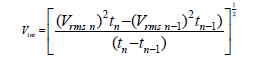
Where,

V_{rms n-1}: RMS velocities on the top of the nth layer.

V_{rms n}: RMS velocities on the bottom of the nth layer.

t_n-1: The zero-offset travel times on the top of the nth layer.

t_n: The zero-offset travel times on the bottom of the nth layer.

Figure 10:2D Interval Seismic Velocity Model for 112-100 Well.

Figure 11:2D Interval Seismic Velocity Model for 112-119 Well.

Figure 12:2D Interval Seismic Velocity Model for 113-16 Well.

Formations thicknesses of layers having different acoustic impedances can be found by multiplication of one-way time differences by interval velocities [2]. Then, depths can be found from the summation of these layer thicknesses (Figure 10-12).

In this study (Eaton’s) method was applied to predict pore pressure before drilling from seismic interval velocities. The Eaton’s method is the most widely used in oil field which based on the under- compaction mechanism and the relation between the effective stresses in abnormal and normal compaction conditions. The overburden stress is a function of depth and is calculated from bulk density by using [6]. where this equation shows that the relationship between the elastic wave velocities and the vertical effective stress.

𝜌=𝑎V^𝛽

Given Gardner’s parameters 𝑎 and 𝛽. With density (g/cm3) and velocity (m/s), typical values of 𝑎 and 𝛽 for Gulf Coast sediments are 𝑎=0.31 and 𝛽=0.25, [6].

Overburden pressure (σ_ovb) is obtained from bulk density using:

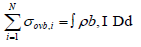
Or

σ_ovb (psi)=0.052 x ρb (lb/gal or ppg) x D (ft)

Where D is the depth of interest.

Through (Eaton’s) method can be estimated the vertical component of the effective stress from seismic velocities by the relationship:

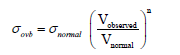
Where σ_normal and V_normal are the vertical effective stress and the seismic velocity expected if the sediment is normally pressured, while 𝑛 is an exponent for the sensitivity of velocity to effective stress [7-10].

The pore pressure is then given by:

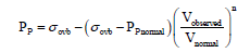
σ_ovb is the overburden stress, 𝑃_{𝑝 𝗇𝗈𝗋𝗆𝖺𝗅} the normal pore pressure, 𝑉_{𝚘𝚋𝚜𝚎𝚛𝚟𝚎𝚍} the seismic velocity, and 𝑉_{𝗇𝗈𝗋𝗆𝖺𝗅} the normal seismic velocity the exponent 𝑛 can be adjusted from well data or may be kept fixed the value 3. Figure 13-20 Shows pore pressure prediction to available wells in the study area.

Figure 13:2D Interval Seismic Velocity Model for 113-60 Well.

Figure 14:2D Interval Seismic Velocity Model for 113-95 Well.

Figure 15:2D Interval Seismic Velocity Model for 113-112 Well.

Figure 16:2D Interval Seismic Velocity Model for 113-124 Well.

Figure 17:2D Interval Seismic Velocity Model for 113-A-21 Well.

Figure 18:Pore Pressure Prediction from Seismic Velocity for 112-100 Well.

Figure 19:Pore Pressure Prediction from Seismic Velocity for 112-119 Well.

Figure 20:Pore Pressure Prediction from Seismic Velocity for 113-16 Well.

In the third step is constructing 3-D cube for interval velocity, estimated bulk density and pore pressure prediction to show distributions across the study area. Also, constructing pore pressure distribution maps to every formation where we can determine pore pressure distributions within every formation in the study area [11-13].

This study carried out on eight wells are spread across Belayim Land oil field (112-100, 112-119, 113-16, 113-60, 113-95, 113-112, 113-124 and 113-A-21) where the aims of this part to present the results of pore pressure prediction using interval seismic velocity and report any indication of anomaly present in pore pressure prediction and determine mud weight to every interval.

In the first as previously described in methodology, we can extract seismic interval velocity along on wellbores paths for every well, Figure 10-17 Shows interval seismic velocity model to available wells in the study area, the bulk density can be estimated from the interval velocity that obtained by using (Gardener equation). Where we can show that increasing bulk density with increasing interval velocity which reflects the change in the lithology and its effect on interval velocity [14-16].

Overburden pressure is generated from the density log, also Compaction trends are identified for each well based on interval velocity responses. Pre-drill pore pressure prediction for 112- 100 well shows in Figure 18 An NCT was generated where pore pressure prediction trend shows that this well is expected to be normally compacted, or close to normally compacted to +/- 1970m TVDss, then a slight decreasing gradually in pore pressure trend at top of Belayim Formation where it is clear that present a pore pressure depletion where the maximum pore pressure predicted was 7.8ppg EMW. In Kareem Formation pore pressure behavior reaching a value 7.75ppg EMW as the maximum value. In addition, pore pressure which predicted in Rudies Formation was 8ppg EMW. No RFT measurements were taken in this well.

Pre-drill pore pressure prediction for 112-119 well shows in Figure 19 An NCT was generated where pore pressure prediction trend shows that this well is expected to be normal to +/- 2010m TVDss. Also, a slight decreasing in predicted pore pressure trend at top of Belayim Formation as a result of pressure depletion to reach maximum pore pressure 7.8ppg EMW. In Kareem Formation also continuous pressure regression to reach a maximum value of 7.55ppg EMW, while Rudies Formation shows that the maximum value was 7.5ppg EMW.

Pre-drill pore pressure prediction for 113-16 well shows in Figure 20 An NCT was generated where pore pressure prediction trend shows that this well falls on or near normal compaction trend to +/- 2040m TVDss, after that appears to have a different pore pressure regime which appearing decreasing gradually in pore pressure trend at top of Belayim Formation where the maximum pore pressure prediction was 7.85ppg EMW. Then pore pressure decreasing in Kareem Formation to reach a value 7.55ppg EMW. In Rudies Formation pore pressure was predicted to be 8ppg EMW. Unfortunately, there are no measured pressures in this interval.

Pre-drill pore pressure prediction for 113-60 well shows in Figure 21 An NCT was generated where pore pressure prediction trend shows that this well is expected to be normal to +/- 2020m TVDss, this will be followed by a reversal decrease in pore pressure behavior reaching a value of 7.75ppg EMW inside Belayim Formation, where Kareem Formation show that the maximum pore pressure predicted was 7.9ppg EMW while pore pressure prediction trend in Rudies Formation show that the maximum value was 7.8ppg EMW.

Figure 21:Pore Pressure Prediction from Seismic Velocity for 113-60 Well.

Pre-drill pore pressure prediction for 113-95 well shows in Figure 22 An NCT was generated where pore pressure prediction trend of this well is expected to be normally compacted, or close to normally compacted to +/- 1900m TVDss. then a slight decreasing in pore pressure trend which decreases to reach the maximum value of 7.9ppg EMW inside Belayim Formation. Then continuous decreases in predicted pore pressure as a result of pressure depletion in Kareem Formation to reach the maximum value of 7.65ppg EMW. In Rudies Formation show that continuous depletion where the maximum pore pressure predicted was 6.55ppg EMW. So, it is important to mention that a pore pressure depletion, as clear from the RFT’s data [17-19].

Figure 22:Pore Pressure Prediction from Seismic Velocity for 113-95 Well.

Pre-drill pore pressure prediction for 113-112 well shows in Figure 23 An NCT was generated where pore pressure prediction trend of this well is expected to be normal to +/- 1935m TVDss, then show that a reversal decrease in pore pressure in approaching Belayim Formation where it shows that the maximum value was 6.5ppg EMW as result of pressure depletion (Figure 23).

Figure 23:Pore Pressure Prediction from Seismic Velocity for 113-112 Well.

In Kareem Formation, the maximum value of pore pressure prediction was 6.5ppg EMW while in Rudies Formation was 7ppg EMW. Also, this well shows that pressure depletion, as clear from the RFT’s data. Pre-drill pore pressure prediction for 113-124 well shows in Figure 24 An NCT was generated where pore pressure prediction trend of this well is expected to be normal to +/- 1960m TVDss. Then it shows that a pressure regression prediction inside Belayim Formation where the maximum predicted pore pressure was 6ppg EMW which reflect that sharp depletion, also pore pressure prediction in Kareem Formation show that the maximum pore pressure prediction was 5.9ppg EMW. Then pore pressure for Rudies Formation which shows that the maximum pore pressure value was 6.7ppg EMW. Pore pressure predicted was confirmed by the RFT.

Figure 24:Pore Pressure Prediction from Seismic Velocity for 113-124 Well.

Pre-drill pore pressure prediction for 113-A-21 well shows in Figure 25 An NCT was generated where pore pressure prediction trend of this well is expected to be normally compacted, or close to normally compacted to +/- 1900m TVDss , After that appears to have a different pore pressure regime which reflects decreasing in predicted pore pressure as result of pressure depletion where the maximum pore pressure was 7.7ppg EMW in Belayim Formation where the maximum value in Kareem Formation was 7.2ppg EMW, also the maximum pore pressure prediction for Rudies Formation was 7.7ppg EMW. So, it is important to mention that a pore pressure depletion, as clear from the RFT’s data which show that reality of pressure regression.

Figure 25:Pore Pressure Prediction from Seismic Velocity for 113-A-21 Well.

Pore pressure analysis according to (Eaton’s) method to available wells reveals that no major pressure anomaly exists and appears some anomalous zone which led to the deviation of predicted pore pressure where most of these wells were drilled after the field start-up which reflects some pressure depletion where was recorded and encountered in many areas while drilling for oil and gas where pressure depletion may occur artificially by reducing oil, gas, and water from permeable subsurface formations where production of large amounts of reservoir fluids can drastically reduce formation pressure.

Figure 26:3-D View to Interval Seismic Velocity Model.

Figure 27:3-D View to Bulk Density Model.

The predicted pore pressure values were compared with measured pore pressure values using Repeat Formation Tester (RFT) which represented in Yellow Squares and observed an excellent match between them which indicate the reliability of our predicted results. Interval seismic velocity which derived by using horizon-keyed velocity analysis for the main horizons in the section used to build up a grid by computing the interval velocity between main horizons and it gives high-resolution velocity analyses then used to generate interval velocity cube Figure 26 which used to calculate bulk density by using (Gardener equation) from interval seismic velocity then represented in 3-D cube Figure 27.

Pore pressure predicted is presented in 3-D cube Figure 28 Show that pore pressure distributed through the study area where the beauty of 3-D pore pressure cube is that we can predict and extract pore pressure at any point.

Figure 28:3-D View to Pore Pressure Prediction from Interval Seismic Velocity Model.

Pore pressure prediction cube show that are normally compacted, or close to normally compacted and reveal that no major pressure anomaly exists to approximately+/- 1950m TVDss which require and recommend mud weight 8.5ppg to 10.7ppg to drill then shows a pressure regression prediction in the interval with with low pore pressure prediction which represent depleted zone which require and recommend drilling with low mud weight lower than 8.34ppg [20].

Figure 29:Pore Pressure Distribution Map to Belayim Formation.

Figure 30:Pore Pressure Distribution Map to Kareem Formation

Also, pore pressure distribution maps are constructed in the study area which used for determining locations that higherpressure zone and lower pressure zone where the lower pore pressure area represent locations for design future wells. Pore pressure distributed map to Belayim Formation Figure 29 Show that pore pressure increases in the northern east directions and decreases gradually to the southwest direction, while pore pressure distributed map to Kareem Formation Figure 30 Exhibits that pore pressure increases in the northeast direction and decreases gradually to the southwest directions.

Figure 31:Pore Pressure Distribution Map to Rudies Formation.

Also pore pressure distributed map to Rudies Formation Figure 31 exhibits both higher pore pressure and lower pore pressure where pore pressure increases in the northeast direction and decreases gradually towards the north part and in the southwest direction of the study area [21].

In addition, available geological and geophysical data indicate paths for fluid flow. where fault patterns, as interpreted from structure map, have provided conduits for hydrocarbon migration, where it plays role in migration pathways within these formations from the higher-pressure zones to the lower pressure zones, also there are some vertical faults, some of which represent pressure barriers. So that oil and gas have driven and migrated by high pressure and faults into sandstone of low pressure which represent good locations for the hydrocarbons and design the future wells for development plans.

Application of interval seismic velocities for Pre-drill pore pressure prediction not only to drilling plan but also to safe drilling and to minimize drilling risks and reduce the cost of drilling and determine the area for the future wells.

Pore pressure prediction from the seismic survey has been carried out in Belayim Land Oil Field which lies between longitudes 33˚ 12 and 33˚ 15 east and latitudes 28˚ 35 and 28˚ 40 north where seismic interval velocities derived by using horizon-keyed velocity analysis for the main horizons. Bulk density can be calculated from the interval velocity that obtained by using Gardener equation to calculate overburden Pressure, then normal compaction trend was generated by using Eaton’s equation method to predict pore pressure from interval seismic. After that, the predicted pore pressure values were compared with measured pore pressure values using Repeat Formation Tester (RFT) and observed an excellent match between them which indicate the reliability of our predicted results.

Interval seismic velocity which derived by using horizon-keyed velocity analysis, bulk density which calculated by using Gardener equation and pore pressure predicted represented in 3-D cube through the study area where the beauty of 3-D pore pressure cube is that we can predict and extract pore pressure at any point.

Pore pressure prediction cube show that are normally compacted, or close to normally compacted and reveal that no major pressure anomaly exists to approximately+/- 1950m TVDss which require and recommend mud weight 8.5ppg to 10.7ppg to drill then shows a pressure regression prediction in the interval with with low pore pressure prediction which represent depleted zone which require and recommend drilling with low mud weight lower than 8.34ppg.

Pore pressure distribution maps for the studied formations are constructed which provides critical information for pore pressure distribution and the influence of fault patterns on the fluid path which can control on the decision for the design of the future wells.

1. Foster JB, Whalen HE (1966) Estimation of formation pressures from Electrical Surveys - Offshore Louisiana 18(2): 165-171.
2. Pennebaker ES (1968) Seismic data indicate depth magnitude of abnormal pressures. Spring Meeting of Southern District, Texas, pp: 184-191.
3. Al Sharhan A (2003) Petroleum geology and potential Hydrocarbon plays in the Gulf of Suez Rift Basin. AAPG Bulletin 87(1): 143-180.
4. El Diasty W Sh, KE Peters (2014) Genetic classification of oil families in the central and southern sectors of the Gulf of Suez, Egypt. Journal of Petroleum Geology 37(2): 105-126.
5. Dix CH (1955) Seismic velocities from surface measurements. Geophysics 20(1): 68-86.
6. Gardner GH, Gardner LW, Gregory AR (1974) Formation velocity and density - The diagnostic basis for stratigraphic traps. Geophysics 39(6): 770-780.
7. Aki K, Richard PG (1980) Quantitative seismology. Freeman and Co. New York, USA, pp: 385–416.
8. Babu S, Sircar A (2011) A comparative study of predicted and actual pore pressures in Tripura, India. Journal of Petroleum Technology and Alternative Fuels 2(9): 150-160.
9. Brahma J, Sircar A, Karmakar G (2013) Pre-drill pore pressure prediction using seismic velocities data on flank and synclinal part of Atharamura anticline in the Eastern Tripura, India. Journal of Petroleum Exploration and Production Technology 3(2): 93-103.
10. Bourgoyne AT, Millheim KK, Chenevert ME, Young FS (1991) Applied Drilling Engineering. Revised 2nd printing, pp: 246-250
11. Bowers GL (1995) Pore pressure estimation from velocity data, Accounting for overpressure mechanisms besides under compaction. Society of Petroleum Engineering, Drilling and Completion 10(2): 89-95.
12. Chopra S, Huffman A (2006) Velocity determination for pore pressure prediction. CSEG Recorder 3, Conference and Exhibition 31(4): 28-46.
13. Dahlberg EC (1982) Applied hydrodynamics in petroleum exploration. Springer-Verlag, New York Inc, USA, pp: 1-155.
14. Eaton BA (1975) The Equation for Geopressure prediction from well logs. SPE of AIME, Dallas, TX, SPE 5544 September 28- October 1, Dallas, USA, pp: 1-11.
15. ENI SPA (1999) Overpressure evaluation manual. Company Manual, pp: 141-170
16. Grauls D, Cassignol C (1993) Identification of a zone of fluid pressureinduced fractures from log and seismic data - a case history. First Break 11(2): 59-68.
17. Ham HH (1966) A method for estimating formation pressures from Gulf Coast well logs. Gulf Coast Association Geological Society 16: 185-197.
18. Hottman CE, Johnson RK (1965) Estimation of formation pressures from log-derived shale properties. JPT 17(6): 717-722.
19. Rouchet J (1981) Stress fields a key to oil migration. AAPG Bulletin 65(1): 74-85.
20. Sayers CM, Johnson GM, Denyer G (2002) Pre-drill pore-pressure prediction using seismic data. Geophysics 67(4): 1286-1292.
21. Swarbick RE, Huffman AR, Bowers GL (1999) Pressure regimes in sedimentary basins and their prediction, the leading-edge p. 2.1